Plotting in Julia
Warning: The time to first plot can be frustratingly long in Julia because of the JIT compilation.
The three most popular options (as far as I know) in Julia are
- Plots.jl
- Defines an unified interface for plotting
- maps arguments to different plotting "backends"
- PyPlot, GR, PlotlyJS, and many more
- For a complete list of backends: http://docs.juliaplots.org/latest/backends/
- Mapping of attributes to backends: http://docs.juliaplots.org/latest/supported/
- First runs can be slowish. I found the GR backend fastest and most stable.
Gadfly.jl
To demonstrate Gadfly, we will go through an example and compare it to ggplot2.
In [1]:
using RCall
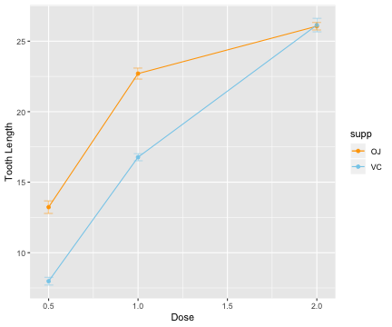
R"""
library(ggplot2)
library(dplyr)
df <- ToothGrowth %>%
group_by(supp, dose) %>%
summarise(se = sd(len) / n(), len = mean(len), n = n())
ggplot(df, aes(x = dose, y = len, group = supp, color = supp)) +
geom_line() +
geom_point() +
geom_errorbar(aes(ymin = len - se, ymax = len + se), width = 0.1, alpha = 0.5,
position = position_dodge(0.005)) +
scale_color_manual(values = c(VC = "skyblue", OJ = "orange")) +
labs(x = "Dose", y = "Tooth Length")
"""
Out[1]:
In [2]:
@rget df # retrieve dataframe from R to Julia workspace
using Gadfly
df[:ymin] = df[:len] - df[:se]
df[:ymax] = df[:len] + df[:se]
Gadfly.plot(df,
    x = :dose,
    y = :len,
    color = :supp,
    Geom.point,
    Guide.xlabel("Dose"),
    Guide.ylabel("Tooth Length"),
    Guide.xticks(ticks = [0.5, 1.0, 1.5, 2.0]),
    Geom.line,
    Geom.errorbar,
    ymin = :ymin,
    ymax = :ymax,
    Scale.color_discrete_manual("orange", "skyblue"))
Out[2]:
Both offer more customized options
In [3]:
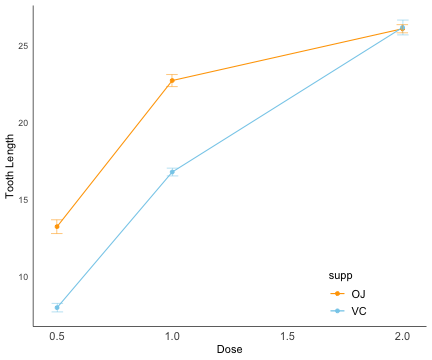
R"""
ggplot(df, aes(x = dose, y = len, group = supp, color = supp)) +
  geom_line() +
  geom_point() +
  geom_errorbar(aes(ymin = len - se, ymax = len + se), width = 0.1, alpha = 0.5,
    position = position_dodge(0.005)) +
    theme(legend.position = c(0.8,0.1),
    legend.key = element_blank(),
    axis.text.x = element_text(angle = 0, size = 11),
    axis.ticks = element_blank(),
    panel.grid.major = element_blank(),
    legend.text=element_text(size = 11),
    panel.border = element_blank(),
    panel.grid.minor = element_blank(),
    panel.background = element_blank(),
    axis.line = element_line(color = 'black',size = 0.3),
  plot.title = element_text(hjust = 0.5)) +
  scale_color_manual(values = c(VC = "skyblue", OJ = "orange")) +
  labs(x = "Dose", y = "Tooth Length")
"""
Out[3]:
In [4]:
Gadfly.plot(df, x = :dose, y = :len, color = :supp, Geom.point,
    Guide.xlabel("Dose"), Guide.ylabel("Tooth Length"),
    Guide.xticks(ticks = [0.5, 1.0, 1.5, 2.0]),
    Theme(panel_fill = nothing, highlight_width = 0mm, point_size = 0.5mm,
    key_position = :inside,
    grid_line_width = 0mm, panel_stroke = colorant"black"),
    Geom.line, Geom.errorbar, ymin = :ymin, ymax = :ymax,
    Scale.color_discrete_manual("orange", "skyblue"))
Out[4]:
Plots.jl
We demonstrate Plots.jl below:
In [5]:
# Pkg.add("Plots")
using Plots, Random

Random.seed!(123) # set seed
x = cumsum(randn(50, 2), dims=1);
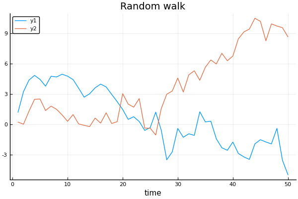
In [6]:
# Pkg.add("PyPlot")
pyplot()  # set the backend to PyPlot
Plots.plot(x, title="Random walk", xlab="time")
Out[6]:
In [7]:
gr()   # change backend to GR
Plots.plot(x, title="Random walk", xlab="time")
Out[7]:
gr()
@gif for i in 1:20
    Plots.plot(x -> sin(x) / (.2i), 0, i, xlim=(0, 20), ylim=(-.75, .75))
    scatter!(x -> cos(x) * .01 * i, 0, i, m=1)
end;
produces following animation.
In [8]:
# Pkg.add("PlotlyJS")
plotlyjs()  # change backend to PlotlyJS
Plots.plot(x, title="Random walk", xlab="time")
Out[8]: