Introduction to

System information (for reproducibility)

In [1]:
versioninfo()
Julia Version 1.4.0
Commit b8e9a9ecc6 (2020-03-21 16:36 UTC)
Platform Info:
  OS: macOS (x86_64-apple-darwin18.6.0)
  CPU: Intel(R) Core(TM) i7-6920HQ CPU @ 2.90GHz
  WORD_SIZE: 64
  LIBM: libopenlibm
  LLVM: libLLVM-8.0.1 (ORCJIT, skylake)
Environment:
  JULIA_EDITOR = code
  JULIA_NUM_THREADS = 4

What's Julia?

Julia is a high-level, high-performance dynamic programming language for technical computing, with syntax that is familiar to users of other technical computing environments

  • History:

    • Project started in 2009. First public release in 2012
    • Creators: Jeff Bezanson, Alan Edelman, Stefan Karpinski, Viral Shah
    • First major release v1.0 was released on Aug 8, 2018
    • Current stable release v1.1.0
  • Aim to solve the notorious two language problem: Prototype code goes into high-level languages like R/Python, production code goes into low-level language like C/C++.

    Julia aims to:

    Walks like Python. Runs like C.
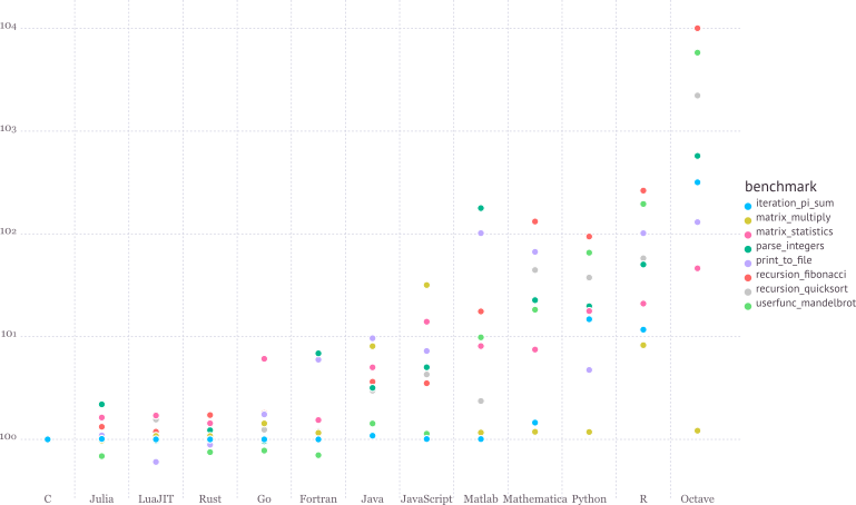
See https://julialang.org/benchmarks/ for the details of benchmark.

  • Write high-level, abstract code that closely resembles mathematical formulas

    • yet produces fast, low-level machine code that has traditionally only been generated by static languages.
  • Julia is more than just "Fast R" or "Fast Matlab"

    • Performance comes from features that work well together.
    • You can't just take the magic dust that makes Julia fast and sprinkle it on [language of choice]

Learning resources

  1. The (free) online course Introduction to Julia, by Jane Herriman.

  2. Cheat sheet: The Fast Track to Julia.

  3. Browse the Julia documentation.

  4. For Matlab users, read Noteworthy Differences From Matlab.

    For R users, read Noteworthy Differences From R.

    For Python users, read Noteworthy Differences From Python.

  5. The Learning page on Julia's website has pointers to many other learning resources.

Julia REPL (Read-Evaluation-Print-Loop)

The Julia REPL, or Julia shell, has at least five modes.

  1. Default mode is the Julian prompt julia>. Type backspace in other modes to enter default mode.

  2. Help mode help?>. Type ? to enter help mode. ?search_term does a fuzzy search for search_term.

  3. Shell mode shell>. Type ; to enter shell mode.

  4. Package mode (@v1.4) pkg>. Type ] to enter package mode for managing Julia packages (install, uninstall, update, ...).

  5. Search mode (reverse-i-search). Press ctrl+R to enter search model.

  6. With RCall.jl package installed, we can enter the R mode by typing $ (shift+4) at Julia REPL.

Some survival commands in Julia REPL:

  1. quit() or Ctrl+D: exit Julia.

  2. Ctrl+C: interrupt execution.

  3. Ctrl+L: clear screen.

  4. Append ; (semi-colon) to suppress displaying output from a command. Same as Matlab.

  5. include("filename.jl") to source a Julia code file.

Seek help

Which IDE?

  • Julia homepage lists many choices: Juno, VS Code, Vim, ...

  • Unfortunately at the moment there are no mature RStudio- or Matlab-like IDE for Julia yet.

  • For dynamic document, e.g., homework, I recommend Jupyter Notebook or JupyterLab.

  • For extensive Julia coding, myself has been happily using the editor VS Code with extensions Julia and VS Code Jupyter Notebook Previewer installed.

Julia package system

  • Each Julia package is a Git repository. Each Julia package name ends with .jl. E.g., Distributions.jl package lives at https://github.com/JuliaStats/Distributions.jl.
    Google search with PackageName.jl usually leads to the package on github.com.

  • The package ecosystem is rapidly maturing; a complete list of registered packages (which are required to have a certain level of testing and documentation) is at http://pkg.julialang.org/.

  • For example, the package called Distributions.jl is added with

    # in Pkg mode
    (@v1.4) pkg> add Distributions
    

    and "removed" (although not completely deleted) with

    # in Pkg mode
    (@v1.4) pkg> rm Distributions
    
  • The package manager provides a dependency solver that determines which packages are actually required to be installed.

  • Non-registered packages are added by cloning the relevant Git repository. E.g.,

    # in Pkg mode
    (@v1.4) pkg> add https://github.com/OpenMendel/SnpArrays.jl
    
  • A package needs only be added once, at which point it is downloaded into your local .julia/packages directory in your home directory.

In [2]:
readdir(Sys.islinux() ? ENV["JULIA_PATH"] * "/pkg/packages" : ENV["HOME"] * "/.julia/packages")
Out[2]:
418-element Array{String,1}:
 ".DS_Store"
 "AMD"
 "AbstractFFTs"
 "AbstractMCMC"
 "AbstractTrees"
 "AccurateArithmetic"
 "Adapt"
 "AlgebraicMultigrid"
 "AlgorithmsFromTheBook"
 "ArgCheck"
 "ArnoldiMethod"
 "Arpack"
 "Arpack_jll"
 ⋮
 "ZMQ"
 "ZeroMQ_jll"
 "ZipFile"
 "Zlib_jll"
 "Zstd_jll"
 "Zygote"
 "ZygoteRules"
 "libass_jll"
 "libfdk_aac_jll"
 "libvorbis_jll"
 "x264_jll"
 "x265_jll"
  • Directory of a specific package can be queried by pathof():
In [3]:
using Distributions

pathof(Distributions)
Out[3]:
"/Users/huazhou/.julia/packages/Distributions/dTXqn/src/Distributions.jl"
  • If you start having problems with packages that seem to be unsolvable, you may try just deleting your .julia directory and reinstalling all your packages.

  • Periodically, one should run update in Pkg mode, which checks for, downloads and installs updated versions of all the packages you currently have installed.

  • status lists the status of all installed packages.

  • Using functions in package.

    using Distributions
    

    This pulls all of the exported functions in the module into your local namespace, as you can check using the whos() command. An alternative is

    import Distributions
    

    Now, the functions from the Distributions package are available only using

    Distributions.<FUNNAME>
    

    All functions, not only exported functions, are always available like this.

Calling R from Julia

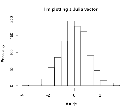
  • The RCall.jl package allows us to embed R code inside of Julia.

  • There are also PyCall.jl, MATLAB.jl, JavaCall.jl, CxxWrap.jl packages for interfacing with other languages.

In [4]:
using RCall

x = randn(1000)
R"""
hist($x, main="I'm plotting a Julia vector")
"""
Out[4]:
RObject{VecSxp}
$breaks
 [1] -4.0 -3.5 -3.0 -2.5 -2.0 -1.5 -1.0 -0.5  0.0  0.5  1.0  1.5  2.0  2.5  3.0
[16]  3.5

$counts
 [1]   1   2   5  21  55  85 134 195 179 163  90  46  15   8   1

$density
 [1] 0.002 0.004 0.010 0.042 0.110 0.170 0.268 0.390 0.358 0.326 0.180 0.092
[13] 0.030 0.016 0.002

$mids
 [1] -3.75 -3.25 -2.75 -2.25 -1.75 -1.25 -0.75 -0.25  0.25  0.75  1.25  1.75
[13]  2.25  2.75  3.25

$xname
[1] "`#JL`$x"

$equidist
[1] TRUE

attr(,"class")
[1] "histogram"
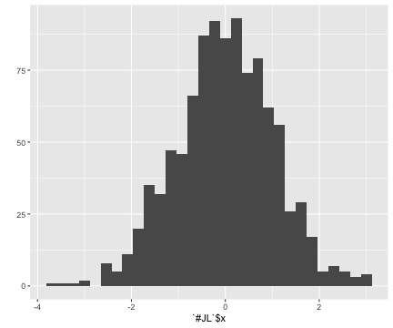
In [5]:
R"""
library(ggplot2)
qplot($x)
"""
Out[5]:
RObject{VecSxp}
┌ Warning: RCall.jl: `stat_bin()` using `bins = 30`. Pick better value with `binwidth`.
└ @ RCall /Users/huazhou/.julia/packages/RCall/g7dhB/src/io.jl:113
In [6]:
x = R"""
rnorm(10)
"""
Out[6]:
RObject{RealSxp}
 [1]  2.113069911 -1.682524682 -0.001947635 -0.188793705 -0.015248555
 [6] -1.076648574  1.077374336  1.274972800 -0.380181292  0.039603064
In [7]:
# collect R variable into Julia workspace
y = collect(x)
Out[7]:
10-element Array{Float64,1}:
  2.113069910576006
 -1.6825246817294395
 -0.0019476347548470132
 -0.18879370539048243
 -0.015248555015719784
 -1.0766485735456024
  1.07737433553574
  1.2749727997552491
 -0.3801812920432254
  0.039603063609110235
  • Access Julia variables in R REPL mode:

    julia> x = rand(5) # Julia variable
    R> y <- $x
    
  • Pass Julia expression in R REPL mode:

    R> y <- $(rand(5))
    
  • Put Julia variable into R environment:

    julia> @rput x
    R> x
    
  • Get R variable into Julia environment:

    R> r <- 2
    Julia> @rget r
    
  • If you want to call Julia within R, check out the XRJulia package by John Chambers.

Some basic Julia code

In [8]:
# an integer, same as int in R
y = 1
typeof(y)
Out[8]:
Int64
In [9]:
# a Float64 number, same as double in R
y = 1.0
typeof(y)
Out[9]:
Float64
In [10]:
# Greek letters:  `\pi<tab>`
π
Out[10]:
π = 3.1415926535897...
In [11]:
typeof(π)
Out[11]:
Irrational{:π}
In [12]:
# Greek letters:  `\theta<tab>`
θ = y + π
Out[12]:
4.141592653589793
In [13]:
# emoji! `\:kissing_cat:<tab>`
😽 = 5.0
Out[13]:
5.0
In [14]:
# `\alpha<tab>\hat<tab>`
α̂ = π
Out[14]:
π = 3.1415926535897...
In [15]:
# vector of Float64 0s
x = zeros(5)
Out[15]:
5-element Array{Float64,1}:
 0.0
 0.0
 0.0
 0.0
 0.0
In [16]:
# vector Int64 0s
x = zeros(Int, 5)
Out[16]:
5-element Array{Int64,1}:
 0
 0
 0
 0
 0
In [17]:
# matrix of Float64 0s
x = zeros(5, 3)
Out[17]:
5×3 Array{Float64,2}:
 0.0  0.0  0.0
 0.0  0.0  0.0
 0.0  0.0  0.0
 0.0  0.0  0.0
 0.0  0.0  0.0
In [18]:
# matrix of Float64 1s
x = ones(5, 3)
Out[18]:
5×3 Array{Float64,2}:
 1.0  1.0  1.0
 1.0  1.0  1.0
 1.0  1.0  1.0
 1.0  1.0  1.0
 1.0  1.0  1.0
In [19]:
# define array without initialization
x = Matrix{Float64}(undef, 5, 3)
Out[19]:
5×3 Array{Float64,2}:
 5.0e-324      5.0e-324  0.0
 6.0e-323      0.0       0.0
 1.0e-323      0.0       0.0
 2.26291e-314  0.0       0.0
 0.0           0.0       0.0
In [20]:
# fill a matrix by 0s
fill!(x, 0)
Out[20]:
5×3 Array{Float64,2}:
 0.0  0.0  0.0
 0.0  0.0  0.0
 0.0  0.0  0.0
 0.0  0.0  0.0
 0.0  0.0  0.0
In [21]:
# initialize an array to be constant 2.5
fill(2.5, (5, 3))
Out[21]:
5×3 Array{Float64,2}:
 2.5  2.5  2.5
 2.5  2.5  2.5
 2.5  2.5  2.5
 2.5  2.5  2.5
 2.5  2.5  2.5
In [22]:
# rational number
a = 3//5
Out[22]:
3//5
In [23]:
typeof(a)
Out[23]:
Rational{Int64}
In [24]:
b = 3//7
Out[24]:
3//7
In [25]:
a + b
Out[25]:
36//35
In [26]:
# uniform [0, 1) random numbers
x = rand(5, 3)
Out[26]:
5×3 Array{Float64,2}:
 0.507598  0.186048   0.628075
 0.989433  0.870866   0.22553
 0.776182  0.189382   0.174717
 0.883318  0.0313765  0.0643843
 0.599743  0.234695   0.42736
In [27]:
# uniform random numbers (in single precision)
x = rand(Float16, 5, 3)
Out[27]:
5×3 Array{Float16,2}:
 0.06445  0.698     0.6523
 0.251    0.3008    0.7363
 0.621    0.3223    0.99
 0.5      0.000977  0.7666
 0.1201   0.542     0.11914
In [28]:
# random numbers from {1,...,5}
x = rand(1:5, 5, 3)
Out[28]:
5×3 Array{Int64,2}:
 3  3  1
 5  3  2
 3  4  2
 1  4  5
 1  5  1
In [29]:
# standard normal random numbers
x = randn(5, 3)
Out[29]:
5×3 Array{Float64,2}:
  0.868721    1.07412    1.14506
  0.352555   -1.0598     0.132082
  0.51563     0.517356  -0.936765
 -0.0663545   0.162099   1.48518
 -0.0847069   1.88382    0.888104
In [30]:
# range
1:10
Out[30]:
1:10
In [31]:
typeof(1:10)
Out[31]:
UnitRange{Int64}
In [32]:
1:2:10
Out[32]:
1:2:9
In [33]:
typeof(1:2:10)
Out[33]:
StepRange{Int64,Int64}
In [34]:
# integers 1-10
x = collect(1:10)
Out[34]:
10-element Array{Int64,1}:
  1
  2
  3
  4
  5
  6
  7
  8
  9
 10
In [35]:
# or equivalently
[1:10...]
Out[35]:
10-element Array{Int64,1}:
  1
  2
  3
  4
  5
  6
  7
  8
  9
 10
In [36]:
# Float64 numbers 1-10
x = collect(1.0:10)
Out[36]:
10-element Array{Float64,1}:
  1.0
  2.0
  3.0
  4.0
  5.0
  6.0
  7.0
  8.0
  9.0
 10.0
In [37]:
# convert to a specific type
convert(Vector{Float64}, 1:10)
Out[37]:
10-element Array{Float64,1}:
  1.0
  2.0
  3.0
  4.0
  5.0
  6.0
  7.0
  8.0
  9.0
 10.0

Matrices and vectors

Dimensions

In [38]:
x = randn(5, 3)
Out[38]:
5×3 Array{Float64,2}:
 -0.0679719  -0.499419     0.464304
 -0.51311     0.391731    -0.276571
  1.51131    -1.37069      0.378619
  1.25128     1.97676     -0.699069
  0.0620681   0.00853839   1.42408
In [39]:
size(x)
Out[39]:
(5, 3)
In [40]:
size(x, 1) # nrow() in R
Out[40]:
5
In [41]:
size(x, 2) # ncol() in R
Out[41]:
3
In [42]:
# total number of elements
length(x)
Out[42]:
15

Indexing

In [43]:
# 5 × 5 matrix of random Normal(0, 1)
x = randn(5, 5)
Out[43]:
5×5 Array{Float64,2}:
 -0.680602   0.612964    0.0529561   0.332952  -0.907096
 -2.17088   -0.713974    0.104878    1.60923   -1.02306
  0.901428  -0.526219    0.29907    -0.254599  -1.16023
  0.108891  -2.5805     -1.36034     0.462398  -0.584862
  1.42368    0.0481646   0.544287    0.178462  -0.278758
In [44]:
# first column
x[:, 1]
Out[44]:
5-element Array{Float64,1}:
 -0.6806017015112786
 -2.170878023180469
  0.9014281956035037
  0.10889141932478424
  1.423675222437071
In [45]:
# first row
x[1, :]
Out[45]:
5-element Array{Float64,1}:
 -0.6806017015112786
  0.6129643293403908
  0.05295607589387902
  0.33295206179339176
 -0.907095749058918
In [46]:
# sub-array
x[1:2, 2:3]
Out[46]:
2×2 Array{Float64,2}:
  0.612964  0.0529561
 -0.713974  0.104878
In [47]:
# getting a subset of a matrix creates a copy, but you can also create "views"
z = view(x, 1:2, 2:3)
Out[47]:
2×2 view(::Array{Float64,2}, 1:2, 2:3) with eltype Float64:
  0.612964  0.0529561
 -0.713974  0.104878
In [48]:
# same as
@views z = x[1:2, 2:3]
Out[48]:
2×2 view(::Array{Float64,2}, 1:2, 2:3) with eltype Float64:
  0.612964  0.0529561
 -0.713974  0.104878
In [49]:
# change in z (view) changes x as well
z[2, 2] = 0.0
x
Out[49]:
5×5 Array{Float64,2}:
 -0.680602   0.612964    0.0529561   0.332952  -0.907096
 -2.17088   -0.713974    0.0         1.60923   -1.02306
  0.901428  -0.526219    0.29907    -0.254599  -1.16023
  0.108891  -2.5805     -1.36034     0.462398  -0.584862
  1.42368    0.0481646   0.544287    0.178462  -0.278758
In [50]:
# y points to same data as x
y = x
Out[50]:
5×5 Array{Float64,2}:
 -0.680602   0.612964    0.0529561   0.332952  -0.907096
 -2.17088   -0.713974    0.0         1.60923   -1.02306
  0.901428  -0.526219    0.29907    -0.254599  -1.16023
  0.108891  -2.5805     -1.36034     0.462398  -0.584862
  1.42368    0.0481646   0.544287    0.178462  -0.278758
In [51]:
# x and y point to same data
pointer(x), pointer(y)
Out[51]:
(Ptr{Float64} @0x00000001165dd490, Ptr{Float64} @0x00000001165dd490)
In [52]:
# changing y also changes x
y[:, 1] .= 0
x
Out[52]:
5×5 Array{Float64,2}:
 0.0   0.612964    0.0529561   0.332952  -0.907096
 0.0  -0.713974    0.0         1.60923   -1.02306
 0.0  -0.526219    0.29907    -0.254599  -1.16023
 0.0  -2.5805     -1.36034     0.462398  -0.584862
 0.0   0.0481646   0.544287    0.178462  -0.278758
In [53]:
# create a new copy of data
z = copy(x)
Out[53]:
5×5 Array{Float64,2}:
 0.0   0.612964    0.0529561   0.332952  -0.907096
 0.0  -0.713974    0.0         1.60923   -1.02306
 0.0  -0.526219    0.29907    -0.254599  -1.16023
 0.0  -2.5805     -1.36034     0.462398  -0.584862
 0.0   0.0481646   0.544287    0.178462  -0.278758
In [54]:
pointer(x), pointer(z)
Out[54]:
(Ptr{Float64} @0x00000001165dd490, Ptr{Float64} @0x000000011617e210)

Concatenate matrices

In [55]:
# 3-by-1 vector
[1, 2, 3]
Out[55]:
3-element Array{Int64,1}:
 1
 2
 3
In [56]:
# 1-by-3 array
[1 2 3]
Out[56]:
1×3 Array{Int64,2}:
 1  2  3
In [57]:
# multiple assignment by tuple
x, y, z = randn(5, 3), randn(5, 2), randn(3, 5)
Out[57]:
([-0.07946595327478304 0.5366206902515758 0.1307347273879236; 1.7279696671313747 1.5241267746650093 1.8724583017639604; … ; -0.12094504677379282 0.14661049014819597 0.34087683471834973; 0.19686837885575847 -0.8183917613580928 -0.30594493713762694], [1.5025239642692927 -0.23889787694491535; -0.285007379207401 -0.2892545052687034; … ; -0.7192051824276394 -0.6163762786059073; 0.0014003052026974325 -1.494586453184664], [-1.01305622020185 -0.4749736708134258 … 0.369403295977617 1.465847037042864; -0.7013788710067068 -0.0674974235178728 … 1.718854144356147 -0.28177382391727085; 0.892424382198883 -0.2568741330038262 … -0.3219874137495171 1.6817461231108182])
In [58]:
[x y] # 5-by-5 matrix
Out[58]:
5×5 Array{Float64,2}:
 -0.079466   0.536621   0.130735   1.50252     -0.238898
  1.72797    1.52413    1.87246   -0.285007    -0.289255
  0.793023   1.44182    0.2899    -0.167062    -0.133781
 -0.120945   0.14661    0.340877  -0.719205    -0.616376
  0.196868  -0.818392  -0.305945   0.00140031  -1.49459
In [59]:
[x y; z] # 8-by-5 matrix
Out[59]:
8×5 Array{Float64,2}:
 -0.079466   0.536621    0.130735    1.50252     -0.238898
  1.72797    1.52413     1.87246    -0.285007    -0.289255
  0.793023   1.44182     0.2899     -0.167062    -0.133781
 -0.120945   0.14661     0.340877   -0.719205    -0.616376
  0.196868  -0.818392   -0.305945    0.00140031  -1.49459
 -1.01306   -0.474974    0.329336    0.369403     1.46585
 -0.701379  -0.0674974  -0.0956562   1.71885     -0.281774
  0.892424  -0.256874   -0.131193   -0.321987     1.68175

Dot operation

Dot operation in Julia is elementwise operation, similar to Matlab.

In [60]:
x = randn(5, 3)
Out[60]:
5×3 Array{Float64,2}:
 -1.29425  -0.26645    1.58016
 -2.10411   1.11568   -0.520928
  1.38334  -1.25722   -0.933339
 -0.64551  -1.33595   -1.02398
 -1.35096   0.170744  -0.30874
In [61]:
y = ones(5, 3)
Out[61]:
5×3 Array{Float64,2}:
 1.0  1.0  1.0
 1.0  1.0  1.0
 1.0  1.0  1.0
 1.0  1.0  1.0
 1.0  1.0  1.0
In [62]:
x .* y # same x * y in R
Out[62]:
5×3 Array{Float64,2}:
 -1.29425  -0.26645    1.58016
 -2.10411   1.11568   -0.520928
  1.38334  -1.25722   -0.933339
 -0.64551  -1.33595   -1.02398
 -1.35096   0.170744  -0.30874
In [63]:
x .^ (-2)
Out[63]:
5×3 Array{Float64,2}:
 0.596983  14.0854     0.400493
 0.225872   0.803376   3.68506
 0.522571   0.632673   1.14795
 2.39991    0.560295   0.953705
 0.547914  34.3011    10.4909
In [64]:
sin.(x)
Out[64]:
5×3 Array{Float64,2}:
 -0.962005  -0.263309   0.999956
 -0.861126   0.898211  -0.497685
  0.982481  -0.951236  -0.803612
 -0.601606  -0.972551  -0.854186
 -0.975934   0.169916  -0.303858

Basic linear algebra

In [65]:
x = randn(5)
Out[65]:
5-element Array{Float64,1}:
  0.22752087078790206
  0.06040469380904837
  1.6253138729701064
 -0.5616584061757285
 -0.3163419010248666
In [66]:
using LinearAlgebra
# vector L2 norm
norm(x)
Out[66]:
1.7642539564697661
In [67]:
# same as
sqrt(sum(abs2, x))
Out[67]:
1.7642539564697661
In [68]:
y = randn(5) # another vector
# dot product
dot(x, y) # x' * y
Out[68]:
2.3343380467299286
In [69]:
# same as
x'y
Out[69]:
2.3343380467299286
In [70]:
x, y = randn(5, 3), randn(3, 2)
# matrix multiplication, same as %*% in R
x * y
Out[70]:
5×2 Array{Float64,2}:
 -0.557807   1.71908
 -0.1451     1.63133
 -0.376415  -1.28496
 -0.952232  -0.634984
 -0.181337   2.31377
In [71]:
x = randn(3, 3)
Out[71]:
3×3 Array{Float64,2}:
  0.604551  -0.663884  -0.427566
  0.171046   0.706153   1.02315
 -0.609924   0.250137   1.49812
In [72]:
# conjugate transpose
x'
Out[72]:
3×3 Adjoint{Float64,Array{Float64,2}}:
  0.604551  0.171046  -0.609924
 -0.663884  0.706153   0.250137
 -0.427566  1.02315    1.49812
In [73]:
b = rand(3)
x'b # same as x' * b
Out[73]:
3-element Array{Float64,1}:
  0.0977277195001287
 -0.20812044826774032
  0.7389752569455617
In [74]:
# trace
tr(x)
Out[74]:
2.8088199654743127
In [75]:
det(x)
Out[75]:
0.8667979988514273
In [76]:
rank(x)
Out[76]:
3

Sparse matrices

In [77]:
using SparseArrays

# 10-by-10 sparse matrix with sparsity 0.1
X = sprandn(10, 10, .1)
Out[77]:
10×10 SparseMatrixCSC{Float64,Int64} with 2 stored entries:
  [4, 4]  =  -0.664695
  [7, 9]  =  -0.50595
In [78]:
# dump() in Julia is like str() in R
dump(X)
SparseMatrixCSC{Float64,Int64}
  m: Int64 10
  n: Int64 10
  colptr: Array{Int64}((11,)) [1, 1, 1, 1, 2, 2, 2, 2, 2, 3, 3]
  rowval: Array{Int64}((2,)) [4, 7]
  nzval: Array{Float64}((2,)) [-0.6646953796712529, -0.5059500670834203]
In [79]:
# convert to dense matrix; be cautious when dealing with big data
Xfull = convert(Matrix{Float64}, X)
Out[79]:
10×10 Array{Float64,2}:
 0.0  0.0  0.0   0.0       0.0  0.0  0.0  0.0   0.0      0.0
 0.0  0.0  0.0   0.0       0.0  0.0  0.0  0.0   0.0      0.0
 0.0  0.0  0.0   0.0       0.0  0.0  0.0  0.0   0.0      0.0
 0.0  0.0  0.0  -0.664695  0.0  0.0  0.0  0.0   0.0      0.0
 0.0  0.0  0.0   0.0       0.0  0.0  0.0  0.0   0.0      0.0
 0.0  0.0  0.0   0.0       0.0  0.0  0.0  0.0   0.0      0.0
 0.0  0.0  0.0   0.0       0.0  0.0  0.0  0.0  -0.50595  0.0
 0.0  0.0  0.0   0.0       0.0  0.0  0.0  0.0   0.0      0.0
 0.0  0.0  0.0   0.0       0.0  0.0  0.0  0.0   0.0      0.0
 0.0  0.0  0.0   0.0       0.0  0.0  0.0  0.0   0.0      0.0
In [80]:
# convert a dense matrix to sparse matrix
sparse(Xfull)
Out[80]:
10×10 SparseMatrixCSC{Float64,Int64} with 2 stored entries:
  [4, 4]  =  -0.664695
  [7, 9]  =  -0.50595
In [81]:
# syntax for sparse linear algebra is same as dense linear algebra
β = ones(10)
X * β
Out[81]:
10-element Array{Float64,1}:
  0.0
  0.0
  0.0
 -0.6646953796712529
  0.0
  0.0
 -0.5059500670834203
  0.0
  0.0
  0.0
In [82]:
# many functions apply to sparse matrices as well
sum(X)
Out[82]:
-1.1706454467546732

Control flow and loops

  • if-elseif-else-end
if condition1
    # do something
elseif condition2
    # do something
else
    # do something
end
  • for loop
for i in 1:10
    println(i)
end
  • Nested for loop:
for i in 1:10
    for j in 1:5
        println(i * j)
    end
end

Same as

for i in 1:10, j in 1:5
    println(i * j)
end
  • Exit loop:
for i in 1:10
    # do something
    if condition1
        break # skip remaining loop
    end
end
  • Exit iteration:
for i in 1:10
    # do something
    if condition1
        continue # skip to next iteration
    end
    # do something
end

Functions

  • In Julia, all arguments to functions are passed by reference, in contrast to R and Matlab.

  • Function names ending with ! indicates that function mutates at least one argument, typically the first.

    sort!(x) # vs sort(x)
    
  • Function definition

function func(req1, req2; key1=dflt1, key2=dflt2)
    # do stuff
    return out1, out2, out3
end

Required arguments are separated with a comma and use the positional notation.
Optional arguments need a default value in the signature.
Semicolon is not required in function call.
return statement is optional.
Multiple outputs can be returned as a tuple, e.g., return out1, out2, out3.

  • Anonymous functions, e.g., x -> x^2, is commonly used in collection function or list comprehensions.

    map(x -> x^2, y) # square each element in x
    
  • Functions can be nested:

function outerfunction()
    # do some outer stuff
    function innerfunction()
        # do inner stuff
        # can access prior outer definitions
    end
    # do more outer stuff
end
  • Functions can be vectorized using the Dot syntax:
In [83]:
# defined for scalar
function myfunc(x)
    return sin(x^2)
end

x = randn(5, 3)
myfunc.(x)
Out[83]:
5×3 Array{Float64,2}:
 0.166046    0.301768   0.0391553
 0.889782    0.0197388  0.95851
 0.333145    0.203833   0.377999
 0.465292    0.102677   0.0260136
 0.0223636  -0.451376   0.899379
  • Collection function (think this as the series of apply functions in R).

    Apply a function to each element of a collection:

map(f, coll) # or
map(coll) do elem
    # do stuff with elem
    # must contain return
end
In [84]:
map(x -> sin(x^2), x)
Out[84]:
5×3 Array{Float64,2}:
 0.166046    0.301768   0.0391553
 0.889782    0.0197388  0.95851
 0.333145    0.203833   0.377999
 0.465292    0.102677   0.0260136
 0.0223636  -0.451376   0.899379
In [85]:
map(x) do elem
    elem = elem^2
    return sin(elem)
end
Out[85]:
5×3 Array{Float64,2}:
 0.166046    0.301768   0.0391553
 0.889782    0.0197388  0.95851
 0.333145    0.203833   0.377999
 0.465292    0.102677   0.0260136
 0.0223636  -0.451376   0.899379
In [86]:
# Mapreduce
mapreduce(x -> sin(x^2), +, x)
Out[86]:
4.354325467105569
In [87]:
# same as
sum(x -> sin(x^2), x)
Out[87]:
4.354325467105569
  • List comprehension
In [88]:
[sin(2i + j) for i in 1:5, j in 1:3] # similar to Python
Out[88]:
5×3 Array{Float64,2}:
  0.14112   -0.756802  -0.958924
 -0.958924  -0.279415   0.656987
  0.656987   0.989358   0.412118
  0.412118  -0.544021  -0.99999
 -0.99999   -0.536573   0.420167

Type system

  • Every variable in Julia has a type.

  • When thinking about types, think about sets.

  • Everything is a subtype of the abstract type Any.

  • An abstract type defines a set of types

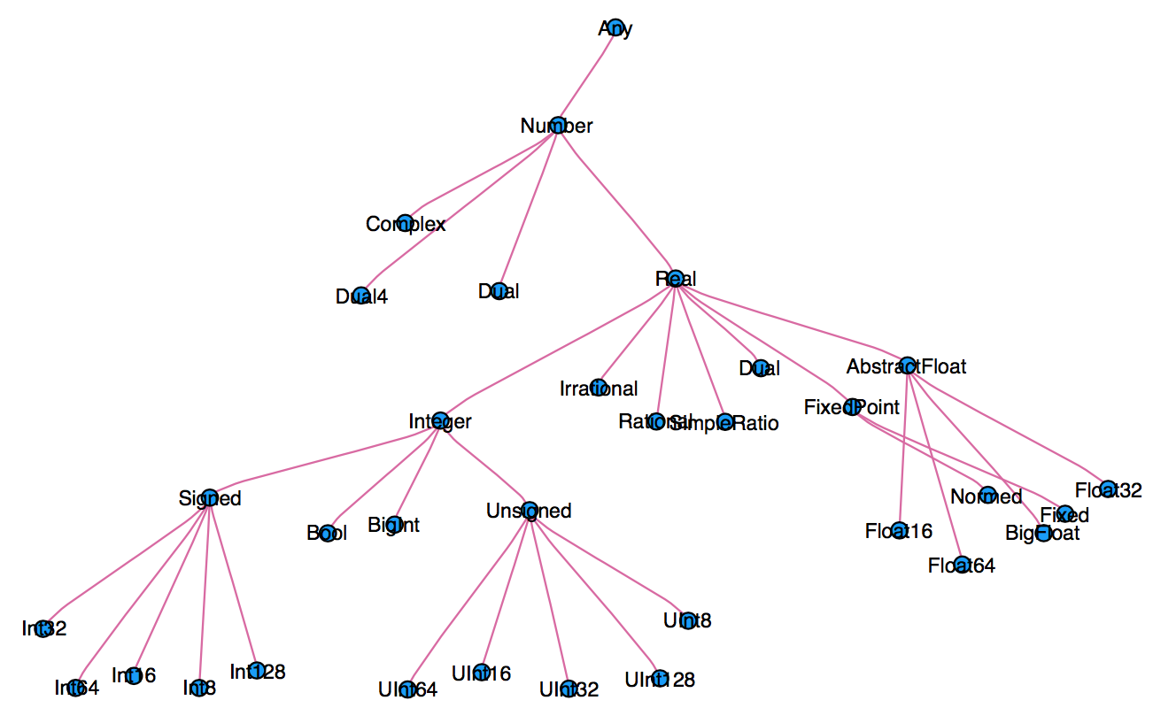
    • Consider types in Julia that are a Number:

  • We can explore type hierarchy with typeof(), supertype(), and subtypes().
In [89]:
typeof(1.0), typeof(1)
Out[89]:
(Float64, Int64)
In [90]:
supertype(Float64)
Out[90]:
AbstractFloat
In [91]:
subtypes(AbstractFloat)
Out[91]:
4-element Array{Any,1}:
 BigFloat
 Float16
 Float32
 Float64
In [92]:
# Is Float64 a subtype of AbstractFloat?
Float64 <: AbstractFloat
Out[92]:
true
In [93]:
# On 64bit machine, Int == Int64
Int == Int64
Out[93]:
true
In [94]:
# convert to Float64
convert(Float64, 1)
Out[94]:
1.0
In [95]:
# same as
Float64(1)
Out[95]:
1.0
In [96]:
# Float32 vector
x = randn(Float32, 5)
Out[96]:
5-element Array{Float32,1}:
 -0.69296366
  0.25062925
 -1.6592916
  0.022112986
  0.71937364
In [97]:
# convert to Float64
convert(Vector{Float64}, x)
Out[97]:
5-element Array{Float64,1}:
 -0.6929636597633362
  0.2506292462348938
 -1.6592916250228882
  0.02211298607289791
  0.7193736433982849
In [98]:
# same as
Float64.(x)
Out[98]:
5-element Array{Float64,1}:
 -0.6929636597633362
  0.2506292462348938
 -1.6592916250228882
  0.02211298607289791
  0.7193736433982849
In [99]:
# convert Float64 to Int64
convert(Int, 1.0)
Out[99]:
1
In [100]:
convert(Int, 1.5) # should use round(1.5)
InexactError: Int64(1.5)

Stacktrace:
 [1] Int64 at ./float.jl:710 [inlined]
 [2] convert(::Type{Int64}, ::Float64) at ./number.jl:7
 [3] top-level scope at In[100]:1
In [101]:
round(Int, 1.5)
Out[101]:
2

Multiple dispatch

  • Multiple dispatch lies in the core of Julia design. It allows built-in and user-defined functions to be overloaded for different combinations of argument types.

  • Let's consider a simple "doubling" function:

In [102]:
g(x) = x + x
Out[102]:
g (generic function with 1 method)
In [103]:
g(1.5)
Out[103]:
3.0

This definition is too broad, since some things, e.g., strings, can't be added

In [104]:
g("hello world")
MethodError: no method matching +(::String, ::String)
Closest candidates are:
  +(::Any, ::Any, !Matched::Any, !Matched::Any...) at operators.jl:529

Stacktrace:
 [1] g(::String) at ./In[102]:1
 [2] top-level scope at In[104]:1
  • This definition is correct but too restrictive, since any Number can be added.
In [105]:
g(x::Float64) = x + x
Out[105]:
g (generic function with 2 methods)
  • This definition will automatically work on the entire type tree above!
In [106]:
g(x::Number) = x + x
Out[106]:
g (generic function with 3 methods)

This is a lot nicer than

function g(x)
    if isa(x, Number)
        return x + x
    else
        throw(ArgumentError("x should be a number"))
    end
end
  • methods(func) function display all methods defined for func.
In [107]:
methods(g)
Out[107]:
# 3 methods for generic function g:
  • g(x::Float64) in Main at In[105]:1
  • g(x::Number) in Main at In[106]:1
  • g(x) in Main at In[102]:1
  • When calling a function with multiple definitions, Julia will search from the narrowest signature to the broadest signature.

  • @which func(x) marco tells which method is being used for argument signature x.

In [108]:
# an Int64 input
@which g(1)
Out[108]:
g(x::Number) in Main at In[106]:1
In [109]:
# a Vector{Float64} input
@which g(randn(5))
Out[109]:
g(x) in Main at In[102]:1

Just-in-time compilation (JIT)

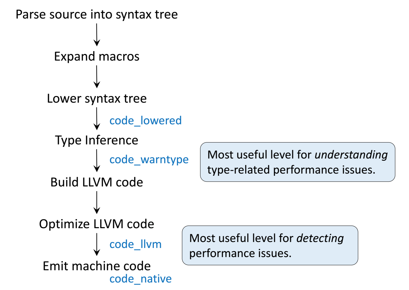
Following figures are taken from Arch D. Robinson's slides Introduction to Writing High Performance Julia.
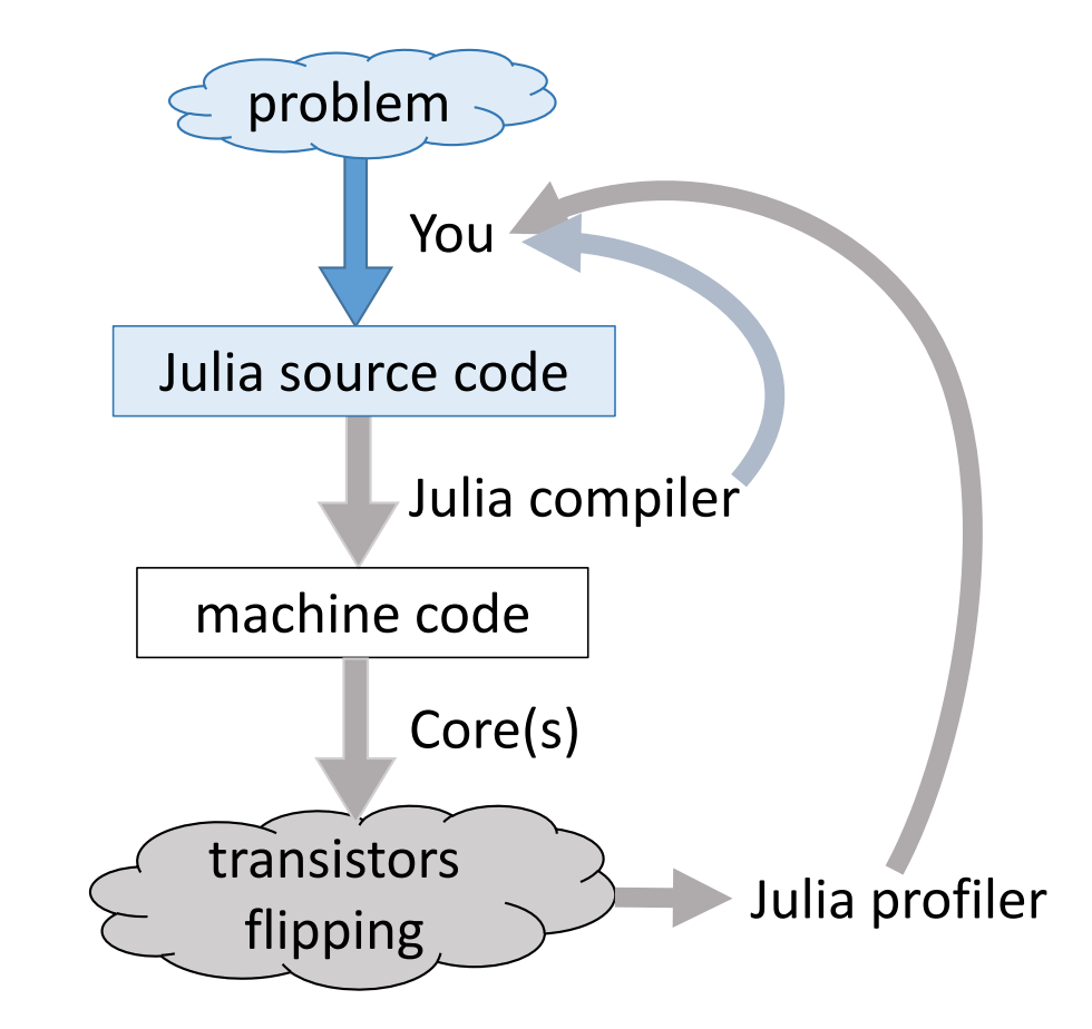
Julia toolchain Julia toolchain
  • Julia's efficiency results from its capability to infer the types of all variables within a function and then call LLVM to generate optimized machine code at run-time.

Consider the g (doubling) function defined earlier. This function will work on any type which has a method for +.

In [110]:
g(2), g(2.0)
Out[110]:
(4, 4.0)

Step 1: Parse Julia code into abstract syntax tree (AST).

In [111]:
@code_lowered g(2)
Out[111]:
CodeInfo(
1 ─ %1 = x + x
└──      return %1
)

Step 2: Type inference according to input type.

In [112]:
@code_warntype g(2)
Variables
  #self#::Core.Compiler.Const(g, false)
  x::Int64

Body::Int64
1 ─ %1 = (x + x)::Int64
└──      return %1
In [113]:
@code_warntype g(2.0)
Variables
  #self#::Core.Compiler.Const(g, false)
  x::Float64

Body::Float64
1 ─ %1 = (x + x)::Float64
└──      return %1

Step 3: Compile into LLVM bytecode (equivalent of R bytecode generated by compiler package).

In [114]:
@code_llvm g(2)
;  @ In[106]:1 within `g'
define i64 @julia_g_19487(i64) {
top:
; ┌ @ int.jl:53 within `+'
   %1 = shl i64 %0, 1
; └
  ret i64 %1
}
In [115]:
@code_llvm g(2.0)
;  @ In[105]:1 within `g'
define double @julia_g_19488(double) {
top:
; ┌ @ float.jl:401 within `+'
   %1 = fadd double %0, %0
; └
  ret double %1
}

We didn't provide a type annotation. But different LLVM code gets generated depending on the argument type!

In R or Python, g(2) and g(2.0) would use the same code for both.

In Julia, g(2) and g(2.0) dispatches to optimized code for Int64 and Float64, respectively.

For integer input x, LLVM compiler is smart enough to know x + x is simple shifting x by 1 bit, which is faster than addition.

  • Step 4: Lowest level is the assembly code, which is machine dependent.
In [116]:
@code_native g(2)
	.section	__TEXT,__text,regular,pure_instructions
; ┌ @ In[106]:1 within `g'
; │┌ @ In[106]:1 within `+'
	leaq	(%rdi,%rdi), %rax
; │└
	retq
	nopw	%cs:(%rax,%rax)
	nop
; └
In [117]:
@code_native g(2.0)
	.section	__TEXT,__text,regular,pure_instructions
; ┌ @ In[105]:1 within `g'
; │┌ @ In[105]:1 within `+'
	vaddsd	%xmm0, %xmm0, %xmm0
; │└
	retq
	nopw	%cs:(%rax,%rax)
	nop
; └

Profiling Julia code

Julia has several built-in tools for profiling. The @time marco outputs run time and heap allocation.

In [118]:
# a function defined earlier
function tally(x::Array)
    s = zero(eltype(x))
    for v in x
        s += v
    end
    s
end

using Random
Random.seed!(123)
a = rand(20_000_000)
@time tally(a) # first run: include compile time
  0.034518 seconds (5.43 k allocations: 251.211 KiB)
Out[118]:
1.0000233387279043e7
In [119]:
@time tally(a)
  0.025372 seconds (1 allocation: 16 bytes)
Out[119]:
1.0000233387279043e7

For more robust benchmarking, the BenchmarkTools.jl package is highly recommended.

In [120]:
using BenchmarkTools

@benchmark tally($a)
Out[120]:
BenchmarkTools.Trial: 
  memory estimate:  0 bytes
  allocs estimate:  0
  --------------
  minimum time:     22.857 ms (0.00% GC)
  median time:      24.148 ms (0.00% GC)
  mean time:        24.326 ms (0.00% GC)
  maximum time:     28.404 ms (0.00% GC)
  --------------
  samples:          206
  evals/sample:     1

The Profile module gives line by line profile results.

In [121]:
using Profile

Profile.clear()
@profile tally(a)
Profile.print(format=:flat)
 Count  Overhead File                    Line Function
 =====  ======== ====                    ==== ========
  1450         0 In[118]                    5 tally(::Array{Float64,1})
     1         1 @Base/abstractdict.jl    638 _oidd_nextind
     1         0 @Base/abstractdict.jl    641 iterate
     2         0 @Base/array.jl           394 getindex
  1450         0 @Base/array.jl           763 iterate
     1         0 @Base/array.jl           914 push!
     1         1 @Base/array.jl           825 setindex!
     2         2 @Base/boot.jl            405 Array
     2         0 @Base/boot.jl            424 Array
  1594       138 @Base/boot.jl            331 eval
     1         0 .../inferenceresult.jl    12 InferenceResult
     1         1 .../inferenceresult.jl    64 matching_cache_argtypes(::Core....
     1         0 ...r/inferencestate.jl   106 Core.Compiler.InferenceState(::...
     1         0 ...r/inferencestate.jl   116 Core.Compiler.InferenceState(::...
     3         0 ...ompiler/optimize.jl   169 optimize(::Core.Compiler.Optimi...
     2         0 ...ler/ssair/driver.jl   107 just_construct_ssa(::Core.CodeI...
     2         0 ...ler/ssair/driver.jl   112 run_passes(::Core.CodeInfo, ::I...
     1         0 ...ler/ssair/driver.jl   121 run_passes(::Core.CodeInfo, ::I...
     1         0 ...ler/ssair/passes.jl   725 getfield_elim_pass!(::Core.Comp...
     1         0 ...r/ssair/slot2ssa.jl   595 construct_ssa!(::Core.CodeInfo,...
     1         0 ...r/ssair/slot2ssa.jl   868 construct_ssa!(::Core.CodeInfo,...
     1         0 ...r/ssair/slot2ssa.jl   378 domsort_ssa!(::Core.Compiler.IR...
     1         1 ...mpiler/typeinfer.jl   126 cache_result(::Core.Compiler.In...
     3         0 ...mpiler/typeinfer.jl    33 typeinf(::Core.Compiler.Inferen...
     1         0 ...mpiler/typeinfer.jl    67 typeinf(::Core.Compiler.Inferen...
     2         0 ...mpiler/typeinfer.jl   572 typeinf_ext(::Core.MethodInstan...
     4         0 ...mpiler/typeinfer.jl   574 typeinf_ext(::Core.MethodInstan...
     6         0 ...mpiler/typeinfer.jl   605 typeinf_ext(::Core.MethodInstan...
  1594         0 @Base/essentials.jl      712 #invokelatest#1
  1594         0 @Base/essentials.jl      711 invokelatest
  1450      1450 @Base/int.jl             409 <
  1450         0 @Base/int.jl             416 <
  1594         0 @Base/task.jl            358 (::IJulia.var"#15#18")()
  1594         0 ...ia/src/eventloop.jl     8 eventloop(::ZMQ.Socket)
  1594         0 .../execute_request.jl    67 execute_request(::ZMQ.Socket, :...
  1594         0 .../SoftGlobalScope.jl   218 softscope_include_string(::Modu...
Total snapshots: 6409

One can use ProfileView package for better visualization of profile data:

using ProfileView

ProfileView.view()
In [122]:
# check type stability
@code_warntype tally(a)
Variables
  #self#::Core.Compiler.Const(tally, false)
  x::Array{Float64,1}
  s::Float64
  @_4::Union{Nothing, Tuple{Float64,Int64}}
  v::Float64

Body::Float64
1 ─ %1  = Main.eltype(x)::Core.Compiler.Const(Float64, false)
       (s = Main.zero(%1))
 %3  = x::Array{Float64,1}
       (@_4 = Base.iterate(%3))
 %5  = (@_4 === nothing)::Bool
 %6  = Base.not_int(%5)::Bool
└──       goto #4 if not %6
2 ┄ %8  = @_4::Tuple{Float64,Int64}::Tuple{Float64,Int64}
       (v = Core.getfield(%8, 1))
 %10 = Core.getfield(%8, 2)::Int64
       (s = s + v)
       (@_4 = Base.iterate(%3, %10))
 %13 = (@_4 === nothing)::Bool
 %14 = Base.not_int(%13)::Bool
└──       goto #4 if not %14
3 ─       goto #2
4 ┄       return s
In [123]:
# check LLVM bitcode
@code_llvm tally(a)
;  @ In[118]:3 within `tally'
define double @julia_tally_19666(%jl_value_t addrspace(10)* nonnull align 16 dereferenceable(40)) {
top:
;  @ In[118]:4 within `tally'
; ┌ @ array.jl:763 within `iterate' @ array.jl:763
; │┌ @ array.jl:221 within `length'
    %1 = addrspacecast %jl_value_t addrspace(10)* %0 to %jl_value_t addrspace(11)*
    %2 = bitcast %jl_value_t addrspace(11)* %1 to %jl_array_t addrspace(11)*
    %3 = getelementptr inbounds %jl_array_t, %jl_array_t addrspace(11)* %2, i64 0, i32 1
    %4 = load i64, i64 addrspace(11)* %3, align 8
; │└
   %5 = icmp slt i64 %4, 1
   br i1 %5, label %L43, label %L18

L18:                                              ; preds = %top
; │┌ @ array.jl:787 within `getindex'
    %6 = bitcast %jl_value_t addrspace(11)* %1 to double addrspace(13)* addrspace(11)*
    %7 = load double addrspace(13)*, double addrspace(13)* addrspace(11)* %6, align 8
; └└
  %value_phi413 = load double, double addrspace(13)* %7, align 8
;  @ In[118]:5 within `tally'
; ┌ @ float.jl:401 within `+'
   %8 = fadd double %value_phi413, 0.000000e+00
; └
; ┌ @ array.jl:763 within `iterate'
; │┌ @ int.jl:416 within `<' @ int.jl:409
    %9 = icmp eq i64 %4, 1
; │└
   br i1 %9, label %L43, label %L37

L37:                                              ; preds = %L18, %L37
   %10 = phi i64 [ %value_phi514, %L37 ], [ 1, %L18 ]
   %11 = phi double [ %14, %L37 ], [ %8, %L18 ]
   %value_phi514 = phi i64 [ %13, %L37 ], [ 2, %L18 ]
; │┌ @ array.jl:787 within `getindex'
    %12 = getelementptr inbounds double, double addrspace(13)* %7, i64 %10
; │└
; │┌ @ int.jl:53 within `+'
    %13 = add i64 %value_phi514, 1
; └└
  %value_phi4 = load double, double addrspace(13)* %12, align 8
;  @ In[118]:5 within `tally'
; ┌ @ float.jl:401 within `+'
   %14 = fadd double %11, %value_phi4
; └
; ┌ @ array.jl:763 within `iterate'
; │┌ @ int.jl:416 within `<' @ int.jl:409
    %15 = icmp ult i64 %value_phi514, %4
; │└
   br i1 %15, label %L37, label %L43

L43:                                              ; preds = %L37, %L18, %top
   %value_phi9 = phi double [ 0.000000e+00, %top ], [ %8, %L18 ], [ %14, %L37 ]
; └
;  @ In[118]:7 within `tally'
  ret double %value_phi9
}
In [124]:
@code_native tally(a)
	.section	__TEXT,__text,regular,pure_instructions
; ┌ @ In[118]:4 within `tally'
; │┌ @ array.jl:763 within `iterate' @ array.jl:763
; ││┌ @ In[118]:3 within `length'
	movq	8(%rdi), %rax
; ││└
	testq	%rax, %rax
	jle	L47
; ││┌ @ array.jl:787 within `getindex'
	movq	(%rdi), %rcx
	vxorpd	%xmm0, %xmm0, %xmm0
; │└└
; │ @ In[118]:5 within `tally'
; │┌ @ float.jl:401 within `+'
	vaddsd	(%rcx), %xmm0, %xmm0
; │└
; │┌ @ array.jl:763 within `iterate'
; ││┌ @ int.jl:416 within `<' @ int.jl:409
	cmpq	$1, %rax
; ││└
	je	L46
; └└
; ┌ @ array.jl within `tally'
	movl	$1, %edx
	nop
; └
; ┌ @ In[118]:5 within `tally'
; │┌ @ float.jl:401 within `+'
L32:
	vaddsd	(%rcx,%rdx,8), %xmm0, %xmm0
; │└
; │┌ @ array.jl:763 within `iterate'
; ││┌ @ int.jl:416 within `<' @ int.jl:409
	addq	$1, %rdx
	cmpq	%rax, %rdx
; ││└
	jb	L32
; │└
; │ @ In[118]:7 within `tally'
L46:
	retq
L47:
	vxorps	%xmm0, %xmm0, %xmm0
; │ @ In[118]:7 within `tally'
	retq
	nopw	%cs:(%rax,%rax)
	nop
; └

Exercise: Annotate the loop in tally function by @simd and look for the difference in LLVM bitcode and machine code.

Memory profiling

Detailed memory profiling requires a detour. First let's write a script bar.jl, which contains the workload function tally and a wrapper for profiling.

In [125]:
;cat bar.jl
using Profile

function tally(x::Array)
    s = zero(eltype(x))
    for v in x
        s += v
    end
    s
end

# call workload from wrapper to avoid misattribution bug
function wrapper()
    y = rand(10000)
    # force compilation
    println(tally(y))
    # clear allocation counters
    Profile.clear_malloc_data()
    # run compiled workload
    println(tally(y))
end

wrapper()

Next, in terminal, we run the script with --track-allocation=user option.

In [126]:
#;julia --track-allocation=user bar.jl

The profiler outputs a file bar.jl.51116.mem.

In [127]:
;cat bar.jl.51116.mem
        - using Profile
        - 
        - function tally(x::Array)
        -     s = zero(eltype(x))
        -     for v in x
        -         s += v
        -     end
        -     s
        - end
        - 
        - # call workload from wrapper to avoid misattribution bug
        - function wrapper()
        0     y = rand(10000)
        -     # force compilation
        0     println(tally(y))
        -     # clear allocation counters
        0     Profile.clear_malloc_data()
        -     # run compiled workload
      528     println(tally(y))
        - end
        - 
        - wrapper()
        -